
Similar to financial investing, cloud rate optimization has an important relationship between the concepts of “risk” and “reward.” For rate optimization, addressing “risk” means having flexibility in the commitment instrument(s) to alter coverage when the usage profile changes. This is important because flexibility (or lack thereof) drives the magnitude of the “reward.” This post breaks down commitment flexibility and how this concept should be applied to maximize savings outcomes while minimizing financial risk.
The necessity of commitment flexibility for rate optimization
Commitment discount instruments, including Savings Plans (SPs), Reserved Instances (RIs), and Committed Use Discounts (CUDs), are typically the single greatest lever for reducing cloud spend. Purchasing these instruments involves either a spend- or resource-based commitment over time in return for discounted pricing. Each discount instrument has unique benefits and drawbacks, so it’s crucial to understand the trade-offs when committing.
It’s tempting to fixate on the absolute discount rate of an instrument, but discounts can wildly vary due to a host of factors (e.g., resource type, region, operating system, term, prepayment, etc.). Informed FinOps practitioners understand there are other dimensions to account for, namely commitment flexibility, when they execute a rate optimization strategy.
Commitment flexibility is the ability to change or adapt the commitment when consumption patterns change, either planned or unplanned. Flexibility is key to achieving world-class rate optimization outcomes.
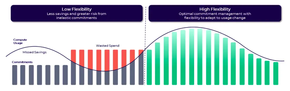
When there is no/low commitment flexibility, users tend to be conservative in the amount of commitment made relative to usage. The result is that more usage is subject to the on-demand rate, and the Effective Savings Rate is below the optimal level (as well as greater Commitment Lock-In Risk).
When there is commitment flexibility, commitment coverage can more closely track the usage patterns in dynamic environments, and the Effective Savings Rate approaches the optimal level (and there is lower Commitment Lock-In Risk).
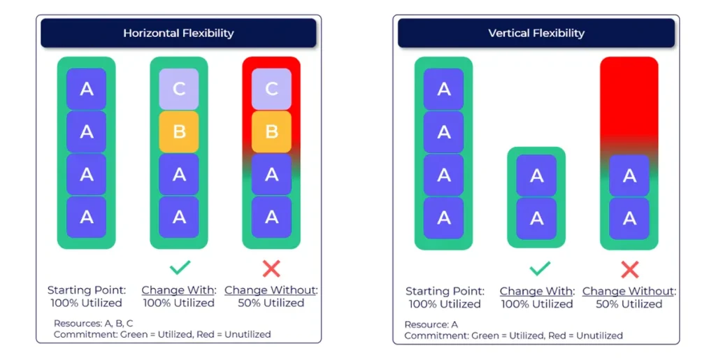
We’ve seen cloud providers also refer to flexibility as a concept, but only focus on one aspect of flexibility (horizontal), when, in fact, there are two dimensions:
1. Horizontal Flexibility (see image below, left)
It means that commitment coverage can “shift” to cover different resource types, based on different attributes, such as instance family, region, OS type, product, etc. Examples of instruments with high horizontal flexibility include AWS and Azure Compute SPs, AWS Convertible RIs, Azure RIs, and Google Cloud spend-based CUDs.
In general, SPs and spend-based CUDs require no human action to adapt to resource type changes, making them highly effective when the mix of resources changes (e.g., r5.xlarge changes to m5.large during weekend lulls). The RI instruments listed above can also adapt horizontally but require active management, making SPs and spend-based CUDs superior for horizontal flexibility.
2. Vertical Flexibility (see image below, right)
It is the ability to increase or decrease the total value of commitment. The only instrument with native vertical flexibility is the AWS Compute Standard RI. Shorter-term commitments can be opportunistically added or removed via the RI Marketplace (within the AWS Terms of Service) to vertically adapt to usage changes. This isn’t automatic and requires management, but the ability to do so fundamentally exists.
Achieving vertical flexibility in all other cases requires various forms of active management to ladder, shift, or otherwise spread commitments over time. In some cases, this is extremely complex, particularly in dynamic environments, and is best accomplished with automation. The primary value of vertical flexibility is to mitigate the risk of overcommitment, where the cost of the commitment exceeds the cost of the underlying usage (e.g., a commitment cost of $5/hr against usage of $3/hr, meaning $2/hour of spend is wasted).
Overcommitment, due to downward movements in consumption, tends to be the greatest risk for cloud users executing a rate optimization strategy and is drastically mitigated when vertical flexibility is successfully implemented.
The best rate optimization outcomes are achieved by blending both dimensions of flexibility.
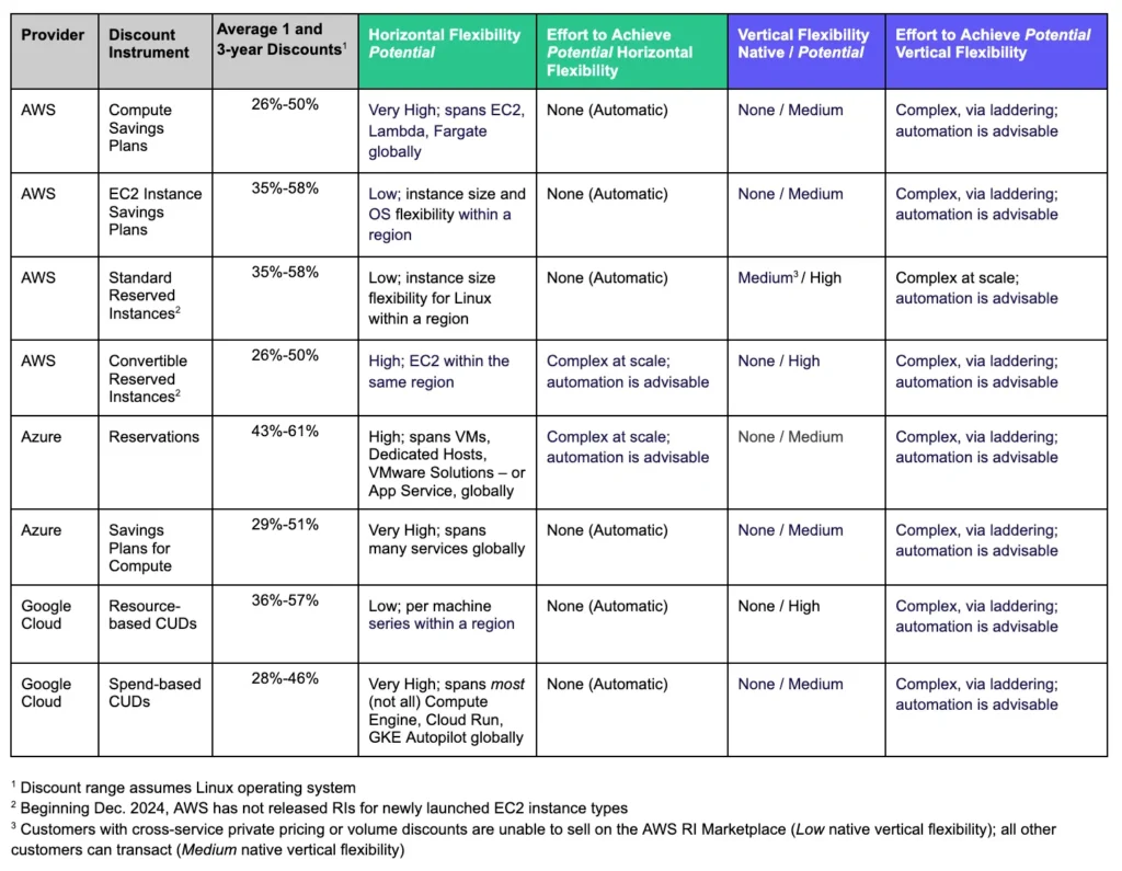
Flexibility across the universe of compute discount instruments
The table below focuses on compute commit discount instruments across clouds. There are non-compute commit discount instruments as well, with various vertical and horizontal properties, but they are not addressed below for purposes of simplicity.
Effective rate optimization strategies should include vertical flexibility
Given these dynamics, ProsperOps algorithms and automation blend instruments that collectively deliver high levels of vertical and horizontal flexibility in order to generate high savings (i.e., achieving a high ESR) while minimizing lock-in (i.e., reducing CLR as much as possible). Because different clouds have discount instruments with different attributes, the implementation tactics change based on the particular cloud and service being optimized. High horizontal flexibility is generally easier to achieve, and in some cases, is automatic. Creating vertical flexibility is hard, but is critical to generating world-class savings outcomes.
Creating vertical flexibility involves advanced RI, SP, and CUD strategies of spreading and shifting commitment over time so that a portion is continually expiring off and/or can be adapted to changes in usage. This safely enables higher coverage with high utilization, which translates into more savings. The exact techniques vary between instruments and clouds, but we call this concept Adaptive Laddering™.
This often involves deploying commitments at high frequency in varying amounts based on observed/forecasted changes in the environment. We wrote on this topic when we released our Savings Plan Adaptive Laddering for AWS Compute feature. Still, Adaptive Laddering concepts are not exclusive to AWS, compute, or Savings Plans. The concepts can be broadly applied (taking advantage of unique cloud/instrument features) to increase vertical flexibility for every rate-optimizable cloud service.
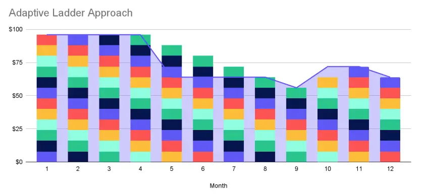
The data shows that more frequent laddering produces higher ESRs over less frequent batch purchases (we’ll cover this in detail in future posts). For example, laddering multiple times per day and dynamically adapting ladder rungs to changes in usage produces better results than monthly or quarterly batch purchases. Implementing ladders may appear straightforward, but manual management, at scale and as part of a dynamic environment, is complicated and time-consuming. A FinOps team would need to continuously perform tasks such as:
- Forecasting detailed usage patterns by resource type and quantity
- Aligning purchases and renewals to track future consumption closely
- Adapting rung purchase sizes and frequencies to dynamic usage changes
- Blending ladders of varying term lengths (e.g., 1- and 3-year commitments)
- Blending a portfolio of ladders that combine discount instruments (e.g., Compute Savings Plans, EC2 Instance Savings Plans, RIs)
- Aligning coverage to the optimal point for cyclical workloads and seasonality
Because commit discount instruments apply hourly, even brief lapses or overlaps in coverage can significantly impact savings. Manual management also increases the risk of human error, resulting in either overcommitting (wasting spend) or undercommitting (incurring higher on-demand costs).
ProsperOps’ mission is to automate FinOps wherever possible, in this case producing higher ESRs (net of our charge), reducing CLRs, freeing up customer FinOps cycles for higher value activities, and generally helping our customers prosper in the cloud.
Schedule a demo if you have questions or want to see our FinOps automation platform in action. Or, request a free savings analysis to quantify your outcomes with ProsperOps.